Preface
Electrical network analysis is an old, mature and seemingly closed subject. Georg Ohm (16 March 1789 - July 1854) published his law in 1827, almost 200 years ago and Gustav Kirchhoff's (12 March 1824 - October 1887) circuit laws date to 1845. One of the more recent advances in network theory is Tellegen's theorem, published by Bernard Tellegen (24 June 1900 - 30 August 1990) in 1952.
But network analysis is far from being a closed subject. It is part of the much broader subject of general network theory which is itself a branch of the mathematical subject of graph theory. This means that many of the powerful methods of graph theory can be applied to electrical network analysis. Once an electrical network has been reduced to a graph we can use the topology, symmetry, and the walk structure of the graph to solve problems related to the underlying electrical network.
Much of the work in this area has not made its way out of the confines of academic research. The electrical engineer is unlikely to be exposed to this way of doing network analysis in their undergraduate education. They may come across some of it in graduate school or later in their career but the practical applications of it may not always be clear. It is our belief that this way of doing network analysis is exciting, interesting and has practical benefits that have yet to be fully realized.
This book is our attempt to bring some of these nonstandard methods of network analysis to the attention of more engineers. In particular, we will show in this book how some of the traditional methods of doing network analysis can be turned into an equivalent problem involving a random walk on a graph. We will show that this probabilistic interpretation of electrical networks leads to graphical techniques that can make it easier to solve circuit analysis problems. The book contains a variety of problems that are solved in detail using this method. We have tried not to make this an academic book. It should be of interest to any engineer looking for new and more efficient ways to do network analysis. The only prerequisite for this book is a good knowledge of standard electrical network theory.
Finally, the website for the book you are now reading is
https://www.abrazol.com/books/rwnet/
where we will post related resources.
Richard Hollos
Exstrom Laboratories LLC
Longmont, Colorado
December 2023
Nodal Analysis with a Voltage Source
When a voltage source is connected across two nodes of a network it will induce voltages at the other nodes. Those other voltages can be found using a method called nodal analysis. We will show how this method works, how it can be used to determine the equivalent admittance or impedance of the network and how it can be turned into a corresponding problem involving a random walk on a graph.
Let's call the number of nodes in the network n + 2. A network must have a minimum of 2 nodes, in which case n = 0. Label the nodes from 0 to n + 1 with the voltage source connected between nodes 0 and n + 1 such that node n + 1 is the ground node (at zero potential). The nodes to which the source is not connected are labeled from 1 to n.
Suppose node 0 (the source node) is connected to m other nodes through admittances Y01,Y02,...,Y0m as shown in figure (1). There will be other connections to node n + 1 (ground) which are not shown in the figure or else this would be a dead network.
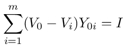
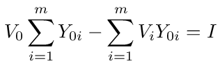
We can find an expression for the equivalent admittance of the network by applying Kirchhoff's current law to node 0. If Vi is the voltage at node i then the current that flows from node 0 to i is given by (V0 - Vi)Y0i. If I is the total current flowing into node 0 from the voltage source, then Kirchhoff's current law tells us that


Figure (1): Voltage source connected to a network.
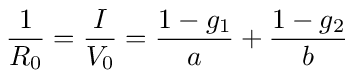
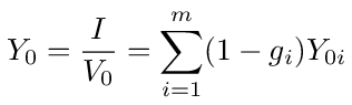
We can get an expression for the equivalent admittance of the network by simply dividing both sides of equation (1) by V0. This gives us the equivalent admittance connected across nodes 0 and n + 1 of the network. Calling this admittance Y0, we have

where gi = Vi/V0 is a voltage transfer function from the source to node i.
To calculate Y0 we still need to find the gi values. We can find them by applying Kirchhoff's current law to the remaining nodes, 1 thru n, of the network (the ground node is not included). This will result in a system of n equations that can then be solved for all the gi, not just the first m required in equation (2).
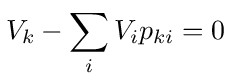
In general for node k, assuming there are no other sources connected to the network, Kirchhoff's current law says that
where the sum is over all nodes connected to node k. The equation simply says that, since there is no source connected to the node, the sum of all currents leaving the node must equal 0. Collecting the Vk terms, we can rewrite equation (3) as follows
For nodes k = 1,2,...,m, one of the nodes connected to k will be node 0 (the source node). If we move that term to the right hand side then equation (4) becomes
Now divide both sides of equations (4) and (5) by
where the sum is over all nodes connected to node k. If we let gk = Vk/V0 be a voltage transfer function and
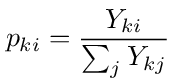
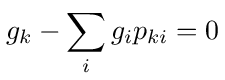
then equation (4), for the nodes that are not connected to node 0, becomes
and equation (5), for the nodes that are connected to node 0, becomes
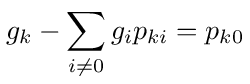
Note that the sum in equation (8) is over all nodes connected to node k and the sum in equation (9) is over all nodes connected to node k except for node 0.
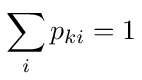
We will call the pki values transition probabilities because in most cases they behave exactly like probabilities. When the Yki are real, i.e. conductances, the pki will be real values less than 1. When the Yki are complex the pki will in general not be real but will have magnitudes less than 1. In both cases the pki are clearly analogous to probabilities in the sense that the sum of all pki for node k will equal 1. Note that when we say all the pki that includes the pki for connections to the ground node which were not used in the formulation of the node equations given above. When connections to the ground node are included we have
When we formulate the network problem as a random walk problem we will see that pki is the probability of jumping from node k to node i.
Before looking at the random walk formulation let's look at the more traditional method of solving the problem. It is clear that equations (8) and (9) must be solved for the voltage transfer functions gi = Vi/V0 which then determine the node voltages Vi given the source voltage V0. The gi values for i = 1 through m can then be used to determine the equivalent admittance of the network via equation (2).
One way to proceed with such a solution is to put equations (8) and (9) into matrix form as follows
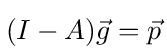
where g⃗ = [g1 g2 ... gn] T is the vector of voltage transfer functions, p⃗ = [p10 ... pm0 0 ... 0] T is the vector of transition probabilities between node 0 and the m nodes connected to it, and A is the transition probability matrix for the network node graph.
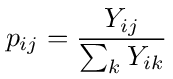
In the current context, the network node graph is a graph where the vertices correspond to nodes 1 to n of the network. Vertex i is connected to vertex j in the graph if node i is connected to node j in the network. The connections are weighted by the transition probabilities and the n by n matrix A tabulates these connections. The element in row i and column j of the matrix A will equal the transition probability pij that connects node i to node j. (From here on we will refer to both the vertices of the graph and the nodes of the network as nodes)
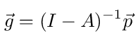
Solving equation (11) for g⃗ involves inverting the matrix I - A. The solution is then
This is a purely abstract formulation of the problem and its solution. We will now analyze a concrete problem in detail which should lead to better understanding of the formalism and how to use it.
Resistive Bridge Circuit
The first network we will analyze is shown in figure (2). It is a simple resistive bridge network with 4 nodes and three unique resistance values: a, b, c. A voltage source is connected between nodes 0 and 3. The problem is to find the voltages at nodes 1 and 2 and the equivalent resistance seen by the voltage source.

Figure (2): Resistive bridge circuit.
If we sum the currents at node 1 we get
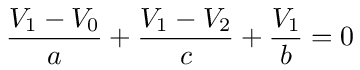
Collecting terms, we can write this as

Now summing the currents at node 2 we get
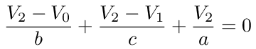
Collecting terms, we can write this as
If we divide equations (14) and (16) by
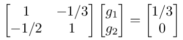
then we get the following system of equations to solve for g1 and g2
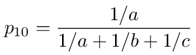
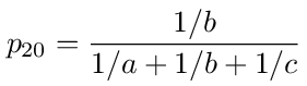
where g1 = V1/V0, g2 = V2/V0, and
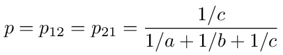
is the transition probability from node 1 to 2 or 2 to 1. On the right hand side we have the transition probabilities from nodes 1 and 2 to the source, node 0.
In matrix form equation (19) is
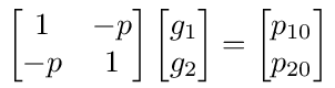
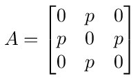
The network node graph for this problem is rather simple, consisting of only nodes 1 and 2 connected to each other. Comparing equation (22) with equation (11) we see that the transition probability matrix is
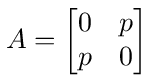
This matrix says that, leaving out the source and ground nodes, the network only consists of two nodes, 1 and 2, connected to each other with transition probability p.
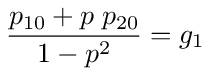
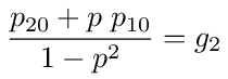
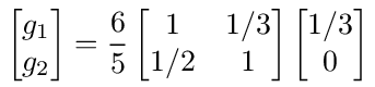
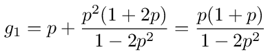
The matrix (I - A) in equation (22) can be easily inverted to give the following solution
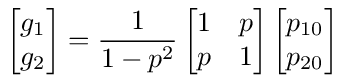
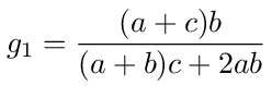
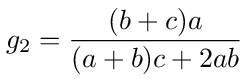
So we have
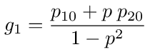
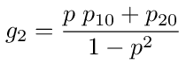
These are the voltage transfer functions g1 = V1/V0 and g2 = V2/V0. Given V0 they give us the voltages V1 and V2. Using the expressions in equations (19), (20) and (21) we have
and when V0 = 1 the voltage across the resistance c is
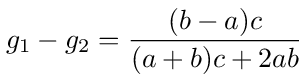
We can see that when a = b there is no voltage across the resistor and g1 = g2 = 1/2 as we would expect.
The g1 and g2 values can now be used to find the equivalent resistance of the network. If we sum the currents at node 0 we get
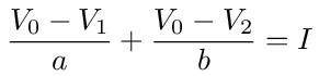
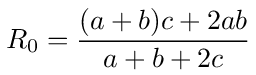
where I is the current flowing into the network from the voltage source. Divide both sides of the equation by V0 to get an expression for the equivalent resistance, R0.
Using the values for g1 and g2 given above we get
A Random Walk Interpretation
To see how the resistive bridge circuit problem corresponds to a random walk on a graph consider the graph shown in figure (3). The nodes in the graph mirror the nodes in the circuit in figure (2). All nodes in the circuit are included in the graph except for the ground node. Transition probabilities from nodes 1 to 2 and from 2 to 1 are both equal to p. Transition probabilities from 1 to 0 and 2 to 0 are p10 and p20 respectively. Note that there are no transition probabilities from 0 to 1 or 2. When a random walk reaches 0 it stops.

Figure (3): Bridge circuit graph.
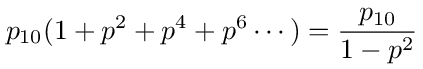
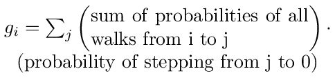
What is the probability that a random walk starting at node 1 ends at node 0? There are two ways to get from 1 to 0. In the first way there will be zero or more round trips from 1 to 2 and back followed by a final step to 0. Each round trip has probability p 2 so the total probability for this way is
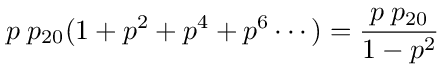
In the second way there will also be zero or more round trips from 1 to 2 and back followed one more step to 2 and a final step to 0. The total probability for this way is
The probability of starting at 1 and ending at 0 will then be the sum of these last two equations
In the same way, we can show that the probability that a random walk starting at node 2 ends at 0 is given by
The probabilities g1 and g2 in equations (35) and (36) are the same as the voltage transfer functions g1 and g2 in equations (25) and (26). If you define the transition probabilities as in equations (19), (20) and (21) then the network problem is identical to this random walk problem.
The general procedure for turning any network problem with a voltage source into a random walk problem is to create a graph for the network that contains all but the ground node. The transition probability going from node i to j in the graph is given by
where Yij is the admittance between i and j and the sum is over all nodes connected to i. There are no transitions out of node 0 (the source node).
The voltage transfer function gi = Vi/V0 is identical to the probability of starting at node i in the graph and ending at node 0. One way to solve for gi is to use the traditional method of constructing the transition probability matrix A that appears in equation (11) where element Ai,j of the matrix is equal to pij. The matrix I - A is inverted to find the vector of voltage transfer functions as in equation (12). The probabilistic interpretation of gi can be seen from the expansion
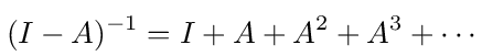
Since element Ai,j (n) of A n is the probability of a walk starting at i and ending at j after n steps the meaning of equation (12) becomes clear. It says that gi is
But matrix inversion is not the only way to calculate g⃗. Individual gi can be calculated using graphical techniques. A simple example of this was shown in the above solution for the resistive bridge network. This is where the real power of turning the network problem into a random walk on a graph becomes apparent. These graphical solution techniques will be demonstrated in more detail in the following examples.
Equal Resistance Ladders
The equal resistance ladder offers one of the most straightforward examples of using the random walk method. The simplest equal resistance ladder is the four resistor network shown in figure (4). The network has four nodes and all resistors have the same value R. A voltage source is connected between nodes 0 and 3. We want to find the voltages at nodes 1 and 2.

Figure (4): 2 rung resistance ladder.
The graph for this network is shown in figure (5). Since node 1 of the network has three equal resistors connected to it, all transition probabilities out of this node in the graph are equal to 1/3. Since node 2 of the network has two equal resistors connected to it, all transition probabilities out of this node in the graph are equal to 1/2. So we have p10 = p12 = 1/3 and p21 = 1/2.

Figure (5): 2 rung ladder graph.
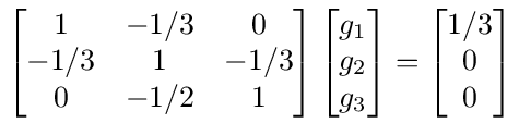
Equation (11) for both the network and graph is then
and the solution using matrix inversion is
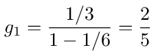
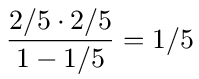
Multiplying this out, we get g1 = 2/5 and g2 = 1/5.
Now we will show another way of arriving at this result using the graphical technique of node elimination. This involves removing a node from the graph and adjusting the connections of the nodes it was connected to so that transition probabilities remain consistent with the original graph. The new transition probabilities are two step probabilities that go through the deleted node. The procedure is best understood with some examples.
We will begin by eliminating node 2 in the graph. Since it is only connected to node 1, it can be eliminated by putting in a loop back transition for node 1 that has probability 1/3 * 1/2 = 1/6 as shown in figure (6). This loop back represents the transition from 1 to 2 and back.
In a walk the loop back transition can be executed any number of times. Therefore, its contribution to the walk probability will be a geometric series in the probability of a single loop. If the probability of a single loop is p then the total contribution of the loop is
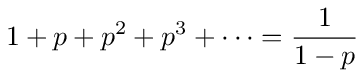
where the p n term in the series represents n loop transitions.

So from figure (6) we see that the probability of a walk starting at 1 and ending at 0 is the loop back transition times the transition probability from 1 to 0 or
This is the same result we got above using matrix inversion.
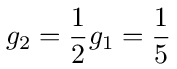
We could now get the probability of starting at 2 and ending at 0 by eliminating node 1 but there is a simpler way. The probability can be found by noting that any walk from 2 to 0 must begin with a step from 2 to 1 with probability 1/2. From there we have a walk that starts at 1 and ends at 0 but we already know that probability. It's g1 which we calculated above. So we have
Which is again the same result found by matrix inversion.
In this particular case we could also find g2 by translating back to the language of voltages. In terms of voltages we have
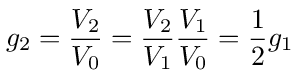
where we have used the fact that V1/V0 = g1 and from the network diagram in figure (4) it is clear that we have a simple voltage divider where V2/V1 = 1/2.
The graphical technique of node elimination that we used here is very powerful. It can be used to calculate some or all of the gi values without the need to invert a matrix. There will be more examples of how it is used in the following problems.
Let's now look at the slightly larger resistance ladder shown in figure (7). The network has five nodes and once again all resistors have the same value R. A voltage source is connected between nodes 0 and 4. We want to find the voltages at nodes 1, 2 and 3.

Figure (7): 3 rung resistance ladder.
The graph for this network is shown in figure (8). Nodes 1 and 2 of the network both have three equal resistors connected to them so all transition probabilities out of these nodes in the graph are equal to 1/3. Node 3 of the network has two equal resistors connected to it so all transition probabilities out of this node in the graph are equal to 1/2. The graph transition probabilities are then p10 = p12 = p21 = p23 = 1/3 and p32 = 1/2.

Figure (8): 3 rung ladder graph.
With these probabilities we can construct the following matrix equation
and the solution using matrix inversion is
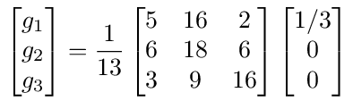
Multiplying this out, we get g1 = 5/13, g2 = 2/13 and g3 = 1/13.
To solve this problem using the graphical method we start by eliminating node 3. This is done by putting a loop back on node 2 as shown in figure (9). The loop back has probability 1/3 * 1/2 = 1/6.

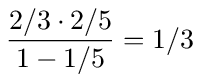
Next we eliminate node 2. This is done by putting a loop back on node 1 as shown in figure (10). To find the probability of this loop back, note that it involves a step from 1 to 2 with probability 1/3 followed by the loop back on 2 which has weight 1/(1 - 1/6) = 6/5 and ending with a step back to 1 with probability 1/3. The loop back probability on node 1 is therefore 1/3 * 6/5 * 1/3 = 2/15.

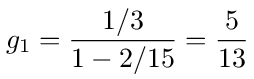
From figure (10) we see that g1 is given by the loop back on node 1 followed by the transition to 0 with probability 1/3.
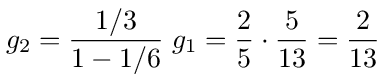
To calculate g2, note that it is the probability of moving from 2 to 1 times g1. From figure (9) we see that the probability of moving from 2 to 1 is given by loop back on 2 followed by the probability of stepping from 2 to 1. So we have
Finally, g3 is the probability of stepping from 3 to 2 times g2. So we have g3 = 1/2 * g2 = 1/13. These are the same values that we got through matrix inversion but they were found by looking at walks on a graph where the connections between nodes are weighted with probabilities.
The way to extend this to longer ladders should be now be clear. As an exercise try solving for the voltages of a four rung ladder. Show that the four gi values are: g1 = 13/34, g2 = 5/34, g3 = 2/34, g4 = 1/34. Show that for a five rung ladder g1 = 34/89, g2 = 13/89, g3 = 5/89, g4 = 2/89, g5 = 1/89. Do you see a pattern? Can you predict the values for the six rung ladder or the n rung ladder?
Resistance Lattices
A very simple resistance lattice is shown in figure (11). The network has five nodes with all resistors equal except for the two connected from node 1 to 4 and from node 3 to 4. A voltage source is connected between nodes 0 and 4, making 4 the ground node. We want to find the voltages at nodes 1, 2 and 3 as well as the equivalent resistance of the network.

Figure (11): Resistor lattice network.
The graph for this network is shown in figure (12). All the transition probabilities in the graph are equal to p = 1/4. The transition probability matrix is then given by
Calculating the inverse (I - A) -1 we get the following solution for the gi values.
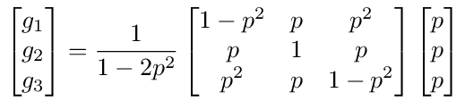
Multiplying this out, we get
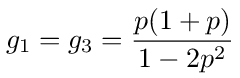
Using the value p = 1/4 we get g1 = g3 = 5/14, g2 = 3/7.

Now let's solve the problem using graphical techniques. From the symmetry of the graph it is clear that g1 = g3 so we will begin by eliminating nodes 1 and 3 to solve for g2.
The loop back probability going from 2 to 1 and back is p 2. This is the same as the loop back probability going from 2 to 3 and back. The total loop back probability on 2, from eliminating 1 and 3, is therefore 2p 2, as shown in figure (13).
With nodes 1 and 3 eliminated the transition probability from 2 to 0 must now include going through 1 or 3 which has probability 2p 2 so the total transition probability going from 2 to 0 is p + 2p 2.
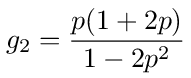
The probability of starting at 2 and ending at 0 is therefore
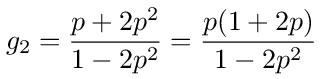
This matches equation (53), calculated by matrix inversion.

Now we want to calculate g1, which is the probability of starting at 1 and ending at 0. We could solve for it using node elimination but we can also get the answer from the value of g2 we just calculated. To start at 1 and end at 0 we can directly transition from 1 to 0 with probability p or we can transition to 2 with probability p and from there end up at 0. This means that g1 = p + pg2. Substituting the value of g2 from equation (54) we get
This matches equation (52), calculated by matrix inversion.
This problem illustrates the fact that, due to the symmetry of the graph, eliminating some nodes first makes the problem easier to solve. To see this, try solving the problem again by first eliminating node 2.
Nodal Analysis with a Current Source
Another way to excite a network is with a current source as shown in figure (14). In this section we will show that such a network can also be analyzed using the random walk method.
As with the voltage source excitation, we will call the number of nodes in the network n + 2. The current source is connected so that current flows into node 0 and we assume that there are m branches coming out of 0 that connect to nodes labeled 1 thru m.

Figure (14): Current source connected to a network.
Applying Kirchhoff's current law to node 0, we get
This is identical to equation (1). The only difference is that now I is the independent variable and all the Vi are dependent variables, including V0. The equation can be written as
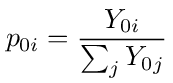
We divide both sides of the equation by ΣiY0i and write it as follows
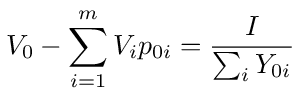
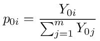
where p0i is the transition probability going from node 0 to i, defined as
For the nodes k ≠ 0 we have

where the sums are over all branches connected to k. Divide both sides of the equation by ΣiYki and write it as follows
where pki is the transition probability going from node k to i, defined as

So there will be n + 1 equations in the unknowns V0,V1,...,Vn. In matrix form the system of equations is written as
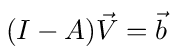
where V⃗ = [V0 V1 ... Vn] T, b⃗ = [I/ΣiY0i 0 ... 0] T and A is the transition probability matrix for the network node graph that includes all but the ground node, i.e. nodes 0 through n. The element in row k and column i of A is equal to pki as given by equation (62).
The solution for V⃗ is then given, at least formally, by
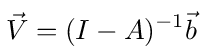
If we let B = (I - A) -1 then since only the first component of the vector b⃗ is nonzero it is clear that the multiplication Bb⃗ in equation (64) results in
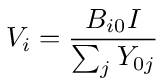
keeping in mind that the admittance summation in the denominator is over all network branches connected to node 0.
In terms of random walks Bi0 is the sum of the probabilities for all random walks that start at node i of the network graph and end at node 0. The sum includes walks of all possible lengths. This probabilistic interpretation for Bi0 becomes clear when we note that B = (I - A) -1 can be expanded as follows
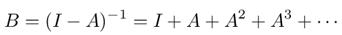
The element in row i and column j of A n is the probability that a walk on the network graph starting at node i will end at node j after exactly n steps. So Bij is the sum of the probabilities for all walks of any length that start at i and end at j.
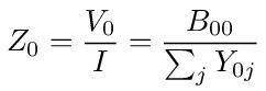
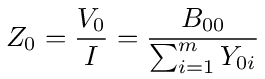
Equation (65) allows us to write the equivalent impedance of the network across nodes 0 and n + 1 as follows
Comparison of Voltage and Current Source Analysis
We have now covered two ways to measure or calculate the equivalent impedance across two nodes of a network. We have shown how to use either a voltage or current source excitation and have given a probabilistic interpretation of both approaches. The remaining thing to do is to show that the probabilistic interpretations are consistent with each other.
When we connected a voltage source across nodes 0 and n + 1 of a network we arrived at equation (2) for the equivalent admittance across the nodes. That equation is repeated here
The sum is over all nodes connected to the source node (0) through admittances Y0i. In terms of voltages, gi = Vi/V0 is a voltage transfer function. In probabilistic terms, gi is the probability that a random walk starting at node i ends at node 0. Recall that the graph on which gi is calculated only has transitions to node 0. There are no transitions away from 0. gi is therefore the probability that when the walk ends at 0 it has not previously visited 0.
Connecting a current source across the same nodes, we arrived at equation (67) for the equivalent impedance across the nodes. That equation is repeated here
The sum is over all nodes connected to the source node (0) through admittances Y0i and, in probabilistic terms, B00 is the sum of the probabilities of random walks of all lengths that start and end at node 0.
To prove the consistency of these two equations we will equate them and show that it leads to a consistent probabilistic interpretation. Equating the two equations, we have
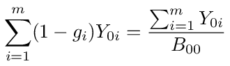
With a bit of rearranging we get
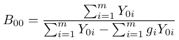
Now divide the top and bottom of this equation by Σi = 1mY0i and write the result as follows
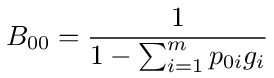
where p0i is the probability of a transition from node 0 to i, given by
With gi being the probability that a walk starts at node i and ends at 0 without any previous visits to 0, it is clear that the sum in the denominator of equation (72), Σi = 1mp0igi, is the probability that a walk starting at node 0 returns there for the first time at the end of the walk. To see this, note that any such walk must begin by transitioning from 0 to one of the i = 1,2,...,m nodes connected to it with probability p0i and from there it will finally return to 0 with probability gi.
Let's call this first return probability f0, then we can write equation (72) as follows
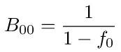
Does this equation make sense from a probabilistic standpoint? If we expand the equation in a power series then it becomes clear that it is probabilistically correct. Expanding in a power series we have
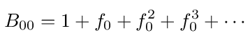
The 1 in the expansion represents a walk that ends at 0 without ever leaving. The f0 term represents a walk that returns to 0 for the first time at the end. The f0 2 term represents a walk that returns to 0 for the second time at the end and so on. These are the probabilities for all the ways that a walk can return to 0 and the sum of these probabilities should be equal to B00 as we have defined it.
Resistive Bridge Circuit With Current Source
For a current source example we will redo the bridge circuit problem with a current source in place of the voltage source as shown in figure (15). The problem is to find the voltages at nodes 0, 1, and 2.

Figure (15): Resistive bridge circuit with current source.
The graph for the network is shown in figure (16). Note that we now have transitions from 0 to 1 and 2 whereas before we only had transitions from 1 and 2 to 0 as seen in figure (3).

Figure (16): Bridge circuit graph.
The A matrix for this network is
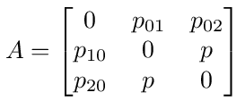
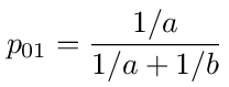
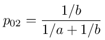
The values for p, p10 and p20 are given by equations (19), (20) and (21). The values for p01 and p02 are given by
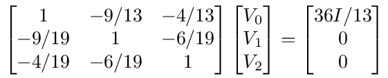
We will now solve the problem using a = 4, b = 9, c = √ab = 6 for which the probabilities are: p = 6/19, p10 = 9/19, p20 = 4/19, p01 = 9/13 and p02 = 4/13. The matrix form of the equation for the node voltages, (I - A)V⃗ = b⃗, is then
and the solution, V⃗ = Bb⃗, where B = (I - A) -1 is
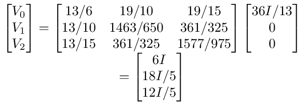
So the equivalent resistance between nodes 0 and 3 is R0 = V0/I = 6.
Now let's see how this can be solved using graphical techniques. If node 2 is eliminated in figure (16) and we use the probabilities listed above then we are left with the graph in figure (17). The 0→0 and 1→1 loop back probabilities are given by
The 0→1 and 1→0 transition probabilities are given by

Finally we eliminate node 1 which leaves only node 0 as shown in figure (18). The loop back probability for node 0 is calculated as follows

From this we can calculate the sum of the probabilities for all walks that start and end at 0
With B00 we can now calculate the voltage at 0
which is the same value we calculated above using matrix inversion.
To get V1 we need B10 which is the sum of the probabilities of all walks that start at 1 and end at 0. That is equal to the probability of looping any number of times at 1 and then moving from 1 to 0 in figure (17) followed by the probability of finally ending at 0. So we have
and the voltage at 1 is then
which is the same value we calculated above using matrix inversion.
To get V2 we need to calculate B20 which we do by eliminating node 1 in figure (16). The resulting graph is shown in figure (19).

B20 is equal to the probability of moving from 2 to 0 in figure (19) followed by the probability of ending at 0. So we have
and the voltage at 2 is then
which is the same value we calculated above using matrix inversion.
Resistor Cube
If you connect resistors along the edges of a cube you get the network shown in figure (20). There are a total of 8 nodes connected by 12 resistors of equal value which we will set equal to 1. Measuring resistances across pairs of nodes, we find that there are only 3 unique values. We have R02, the equivalent resistance across an edge of the cube, R07, the equivalent resistance across the body diagonal of the cube and R05, the equivalent resistance across the face diagonal of the cube.

Figure (20): Resistor cube network.
To measure these resistances we will connect a current source to node 0 and ground node 2 for R02, node 7 for R07 and node 5 for R05. In all three cases it is clear from the symmetry of the network that we will have equal voltages at nodes 4 and 6, V4 = V6, and at nodes 1 and 3, V1 = V3. This means we can connect node 4 with 6 and node 1 with 3 without affecting the overall behavior of the network. If we connect nodes 4 and 6 we get the equivalent network shown in figure (21). If we now connect nodes 1 and 3 we get the equivalent network shown in figure (22).

Figure (21): Resistor cube network with nodes 4 and 6 combined.

From this equivalent network R02 can be found using the standard method of combining series and parallel resistances. Following the node path 4 - 7 - 5 - 1 there are 3 resistances in series that can be combined into a single resistor of value 2. This is in parallel with the resistance 1/2 between nodes 4 and 1. Combining these parallel resistors gives a resistance of 2/5. This leaves us with the network shown in figure (23) from which it is easy to calculate R02. We have a resistance of 7/5 in parallel with a resistance of 1 so we get R02 = 7/12.

Figure (23): The network in figure (22) with nodes 7 and 5 eliminated by combining series and parallel resistances
To get R07 we eliminate nodes 5 and 2 in figure (22) by combining the resistors connected in series through those nodes to get the equivalent network shown in figure (24). This network is identical to the resistance bridge network shown in figure (15) with a = 1/2, b = 3/2 and c = 1/2. R07 can then be calculated using equation (32).

To get R05 we eliminate nodes 2 and 7 in figure (22) by combining the resistors connected in series through those nodes to get the equivalent network shown in figure (25). This network is topologically identical to the resistance bridge network shown in figure (15) but it has different resistance values. The procedure for calculating the equivalent resistance is the same.

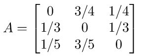
The graph for the network is shown in figure (26) and the A matrix for the network is
The B = (I - A) -1 matrix is
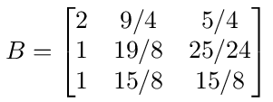
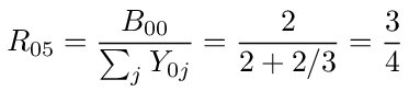
and we get the equivalent resistance using equation (67)
This problem could also be solved using the node elimination techniques we used in previous problems. We leave it as an exercise to solve the problem by eliminating nodes 1 and 4 in the graph to get B00.

Twin-T Notch Filter
The circuit shown in figure (27) is called a twin-T notch filter. The filter input is V0 at node 0 and the output is V3 at node 3. We want to find the voltage transfer function g3 = V3/V0 as a function of frequency and show that it goes to zero when the frequency is equal to 1/2\pi RC.

Figure (27): Twin-T notch filter network.
We will solve this problem using a purely graphical technique. The graph for the network is shown in figure (28). We are driving the network with a voltage source so the voltage at node 0 is fixed and there are only inward transitions, no outward transitions.

Figure (28): Twin-T notch filter graph.
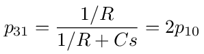
From the network diagram we get the following transition probabilities coming out of node 1.
The transition probabilities coming out of node 2 are:
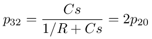
The transition probabilities coming out of node 3 are:

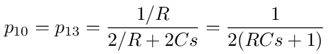
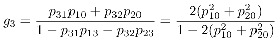
The transfer function g3 = V3/V0 is the probability of a walk starting at node 3 and ending at node 0. We can find this probability by eliminating nodes 1 and 2 so that we are left with only nodes 0 and 3 as shown in figure (29). From the figure we see that g3 is equal to the loop back probability on node 3 followed by the transition to node 0.
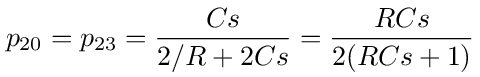
Using the expressions for p10 and p20 given above we have
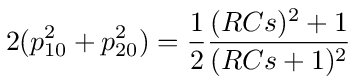
Substituting this into equation (100) and simplifying, we get
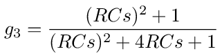
To get the frequency response let s = jω, where j = √-1 then
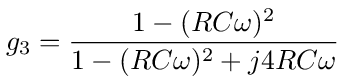
Let RC = 1/ω0 then we can define the dimensionless variable x = ω/ω0 and write the equation as follows
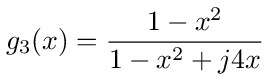

Figure (30): Twin-T frequency response.
The magnitude of the frequency response is then
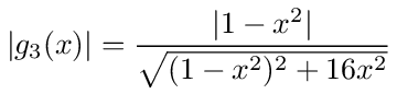
This clearly shows that the twin-T is a notch filter with a zero at x = 1 or ω = ω0 = 1/RC. A plot of the magnitude of the frequency response is shown in figure (30).
Digital to Analog Conversion
As a somewhat more general problem involving multiple voltage sources we will look at the four bit digital to analog conversion circuit shown in figure (31). The four voltage sources b0, b1, b2, b3, can have values that switch between 0 and 1. They are used to represent a four bit binary value. The output value of the circuit is taken from node 3. There should be a total of 16 possible output values corresponding to the 16 binary values represented by the bi sources. In particular we want V3 to be given by the following equation
This input-output relationship is shown in the following table.
| b3b2b1b0 | V3 | b0b1b2b3 | V3 |
|---|---|---|---|
| 0000 | 0 | 1000 | 8/16 |
| 0001 | 1/16 | 1001 | 9/16 |
| 0010 | 2/16 | 1010 | 10/16 |
| 0011 | 3/16 | 1011 | 11/16 |
| 0100 | 4/16 | 1100 | 12/16 |
| 0101 | 5/16 | 1101 | 13/16 |
| 0110 | 6/16 | 1110 | 14/16 |
| 0111 | 7/16 | 1111 | 15/16 |

Figure (31): Four bit digital to analog converter.
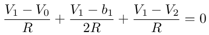
To show that the circuit in figure (31) does satisfy this relationship we will start by using standard nodal analysis on nodes 0 thru 3. For node 0 we have
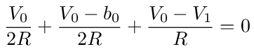
which simplifies to
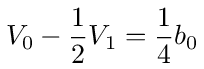
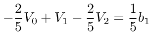
For node 1 we have
which simplifies to
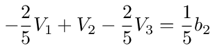
For node 2 we have
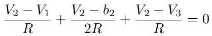
which simplifies to
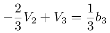
For node 3 we have
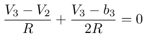
which simplifies to
Equations (108), (110), (112), (114) can be put in matrix form, (I - A)V⃗ = b⃗, as follows
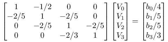
and the solution, V⃗ = Bb⃗, where B = (I - A) -1, is
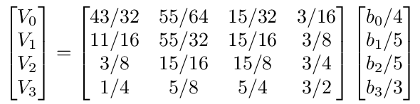
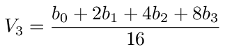
So V3 = b0/16 + b1/8 + b2/4 + b3/2 which is the same as equation (106).
To solve the problem graphically, note that the A matrix in equation (115) represents the transition probability matrix for the linear graph shown in figure (32). To calculate V3 we need the B30, B31, B32, B33 elements of B = (I - A) -1. These are the sums of the probabilities of all walks that start at 3 and end at 0, 1, 2 and 3 respectively.

To calculate B33 we have to eliminate, in order, nodes 0, 1, and 2, leaving only node 3. After eliminating node 0 we are left with the graph in figure (33). The loopback probability on node 1 comes from the transition from 1 to 0 and back again, 2/5 * 1/2 = 1/5.

After eliminating node 1 we are left with the graph in figure (34). The loopback probability on node 2 comes from the transition from 2 to 1, the loop back on 1 and the transition back to 2 again. The calculation is

After eliminating node 2 we are left with only node 3 as shown in figure (35). The loop back probability on 3 is calculated as follows

From this last graph we can write down the value of B33
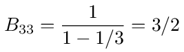
which is the same as the value in full B matrix in equation (116) that was found by inverting (I - A).
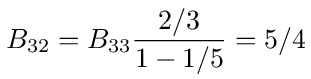
B32 is the sum of the probabilities of all walks starting at 3and ending at 2. Such walks can be decomposed into a walk starting and stopping at 3 followed by a transition to 2 and ending there. So we have
Similarly for B31 and B30 we have
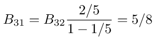
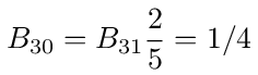
these all match the values in equation (116).
Infinite Networks
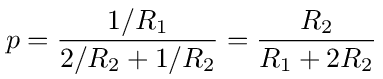
The random walk formalism can be extended to infinite networks such as the infinite length resistance ladder shown in figure (36). The series resistors have value R1 and the shunt resistors have value R2. We will find the equivalent resistance of the network using the voltage source method.
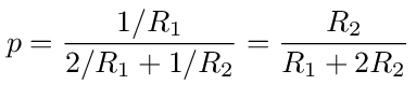
Using the same formalism employed in previous voltage source examples we can get equations for the nodes. For node 1 we get the equation g1 - pg2 = p. For node 2 we get the equation -pg1 + g2 - pg3 = 0, and so on, where gi = Vi/V0 and the transition probability is
All these equations together form an infinite tridiagonal matrix
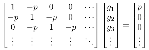

Figure (36): An infinite length resistance ladder.
There are techniques for solving such an equation but we will instead use the graphical technique. The graph for the network is shown in figure (37).

There are an infinite number of nodes in the graph but we can still use node elimination to eliminate all but nodes 0 and 1. This will reduce the graph to that shown in figure (38).

The loop back probability, g, on node 1 is an infinite continued fraction of the following form
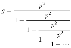
To convince yourself that the probability has this form, try calculating the corresponding probability for a graph with only the nodes explicitly shown in figure (37).
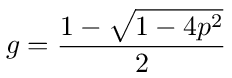
Since this is an infinite continued fraction we can see that the second term in the denominator is itself equal to the g. We can therefor write the equation in the following form

In this form we can solve for g. We find that g is given by
Now from the reduced graph in figure (38) we can write down the expression for g1
Comparing this with equation (126) we see that g1 = g/p or

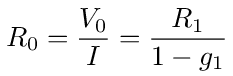
With g1 we can now find the equivalent resistance of the network. If I is the current entering node 0 from the voltage source then
Dividing both sides of this equation by V0 gives us an expression for the equivalent conductance of the network in terms of R1 and g1 = V1/V0. Invert the equation and we have the equivalent resistance of the network.
Substituting the expression for g1 and simplifying we get
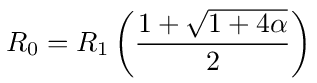
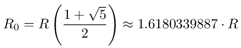
where α = R2/R1.
When R1 = R2 = R then α = 1 and the equivalent resistance is proportional to the golden ratio.
Another infinite network is shown in figure (39). The network has an infinite number of rungs to the right and left of the current source that is driving the network at node 0. We want to find the equivalent resistance looking into node 0.

Figure (39): Two way infinite resistance ladder with current source.
The corresponding graph for this network is shown in figure (40). This is once again an infinite graph with nodes going to plus infinity to the right and negative infinity to the left. All transitions in the graph have probability p given by

The adjacency matrix for the graph is an infinite tridiagonal matrix. Luckily we do not have to calculate the entire B = (I - A) -1 matrix. All we need is the B00 element of the matrix which is the sum of the probabilities for all walks that start and end at node 0. We can find that probability using graphical methods.
Suppose we eliminated all the nodes to the right of node 1 and all the nodes to the left of node -1 then we would be left with the graph in figure (41). The remaining nodes 1 and -1 have loop back probabilities that represent traveling among the eliminated nodes and returning. Clearly, the loop back probability g in figure (40) must be the same as the loop back probability g in figure (38) that was calculated in the previous problem and is given by eq. (127).

Finally we can eliminate nodes -1 and 1, leaving only node 0 with a loop back probability equal to
From this we can write down the expression for B00.
The voltage induced at node 0 by the current source is then
Dividing both sides of this equation by I we get the equivalent resistance looking into node 0
With some substitutions and simplification we have
where α = R2/R1.
As an example, for R1 = R2 = R we have p = 1/3 or α = 1 and
As an exercise show that this is equal to half the resistance in equation (133) in parallel with resistance R. Do you see why this is true?
Transmission Line
When the wavelength of signals in a circuit is much larger than the size of the circuit, the connections between circuit components have little effect. As wavelengths get smaller and become comparable to the size of the circuit the effect of the connections can no longer be ignored and they have to be modeled as transmission lines. A transmission line is essentially a waveguiding structure. Some common examples are coaxial cables and the twin lead used in TV and antenna connections. Traces on circuit boards can also be modeled as transmission lines. What all these structures have in common is that there is a distributed inductance and capacitance down the length of the line. The data sheet for a particular coaxial cable will often list the capacitance per length of the cable and a parameter called the impedance from which the inductance per length can be calculated. If c and l are the capacitance and inductance per unit length then an infinitesimal length dx of the line will have capacitance C = c dx and inductance L = l dx and the entire transmission line can be modeled using the infinite circuit shown in figure (42).

Figure (42): Transmission line model.
This circuit is topologically identical to the infinite length resistance ladder of figure (36) and its graph is identical to the graph shown in figure (37). Since the graph is identical the solution for g1 = V1/V0 will also be given by equation (129) which we repeat below.
But in this case the probability p is equal to
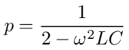
or if we let LC = 1/ω0 2 and x = ω/ω0 then we can write p as
We can use g1 to get the equivalent impedance looking into node 0 of the network. The current entering node 0 is I = (V0 - V1)/jω L so the impedance is
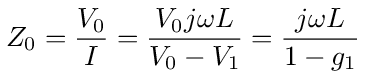
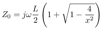
with g1 given by equation (141) and p given by equation (142) we get
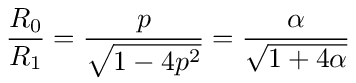
If we split the inductance between nodes 0 and 1 in half then leaving out the first half, the impedance of the rest of the circuit is
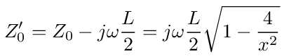
For x<2 or ω<2ω0 the impedance is real so it absorbs energy, while for x>2 or ω>2ω0 the impedance is a pure imaginary number so the entire transmission line looks like a reactance that simply stores energy. Overall then the transmission line looks like a low pass filter. When ω<2/√LC energy is propagated down the line away from the source. When ω>2/√LC energy is stored in the line and not propagated.
We can see this more clearly by looking at the ratio of the voltage from one node to the next. In general the voltage at node n + 1 is related to the voltage at node n as follows: Vn + 1 = Vn - j ω LIn. Since this is an infinite network the impedance looking into each node will be Z0 therefor In = Vn/Z0. Substituting this into the previous equation we see that the voltage ratio from one node to the next remains constant.

With Z0 given by equation (145) and with some simplification we get
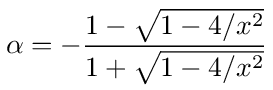
For 4/x 2<1, x>2, ω>2/√LC, α will be real with magnitude less than 1, so the voltage decays going down the line. For 4/x 2>1, x<2, ω<2/√LC, α will be complex with magnitude equal to 1 and phase φ = -2 tan -1√1 - 4/x 2, so α = -e -j φ and the voltage propagates unattenuated down the line with only a change in phase.
The propagation constant in equation (148) can also be found from the network graph. We have α = Vn + 1/Vn = gn + 1/gn and from the graph we can see that the gn must obey the following recurrence equation.
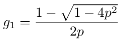
Linear recurrence equations like this can always be solved using the ansatz gn = z n. Substituting this into equation (149) we find that z must satisfy pz 2 - z + p = 0. The solutions to this equation are
Since g1 is given by equation (141), we choose the negative solution to satisfy g1 = z. Therefor we have gn = g1 n and α = gn + 1/gn = g1. With a bit of algebra we can verify that α = g1 is the same as equation (148).
Software
The graphical techniques we used to solve network analysis problems
can easily be implemented in software. For example, in the case of
nodal analysis with a current source we need only one element of the
matrix B = (I - A) -1 where A is the transition probability matrix
for the network node graph. Equation (67) shows that to
calculate the equivalent impedance of a network we need only the upper
leftmost element of the matrix B. Graphically this is equivalent to
eliminating all nodes in the graph except for node 0. The following
function written in the Maxima computer algebra system does exactly
this given the matrix A. Maxima is a free open source computer
algebra system which you can download from
https://maxima.sourceforge.io/
The function is called invert11(A,n) where A is the matrix
and n is the size of the matrix.
invert11(A,n): =
block( [i,j,k],
for i:n thru 2 step -1 do
(
  for j:1 thru i-1 step 1 do
  (
    for k:1 thru i-1 step 1 do
    (
      A[j,k]:A[j,k]+A[j,i]*A[i,k]/(1-A[i,i])
    )
  )
),
return(1/(1-A[1,1]))
);
As an example, we will solve for the equivalent resistance of the resistive bridge circuit in figure (15). The Maxima code for defining the matrix A is
D:a*b+a*c+b*c;
p01:b/(a+b);
p02:a/(a+b);
p10:b*c/D;
p12:a*b/D;
p20:a*c/D;
p21:p12;
A:matrix([0,p01,p02],[p10,0,p12],[p20,p21,0]);
If the function invert11(A,n) is stored in the file
rwen.mac and the above definition of A is stored in the
file bridge2.mac then in a maxima session you would solve for
the equivalent resistance as follows.
load("rwen.mac");
load("bridge2.mac");
ratsimp(invert11(A,3)/(1/a+1/b));
define(f(a,b,c),%);
The function f(a,b,c) defined in the last line will give you the equivalent resistance for any values of a, b, and c. For example, previously we calculated the resistance for a=4, b=9, c=6 so evaluating f(4,9,6) gives 6 which is verified by equation (87).
For a larger example we will solve for the equivalent resistance of the circuit shown in figure (43).

Figure (43): A resistive bridge circuit.
The A matrix for this circuit is defined in Maxima as follows
D0:a*b+a*c+b*c;
D1:a*b+a*r+b*r;
D2:2*b*c+b*r+c*r;
D3:a*c+a*r+c*r;
D4:b*c+b*r+c*r;
D5:2*a*c+a*r+c*r;
p01:b*c/D0;
p02:a*c/D0;
p03:a*b/D0;
p10:b*r/D1;
p12:a*b/D1;
p14:a*r/D1;
p20:c*r/D2;
p21:b*c/D2;
p25:b*r/D2;
p30:a*r/D3;
p32:a*c/D3;
p36:c*r/D3;
p41:c*r/D4;
p45:b*c/D4;
p52:a*r/D5;
p54:a*c/D5;
A:matrix([0,p01,p02,p03,0,0,0],[p10,0,p12,0,p14,0,0],
         [p20,p21,0,p21,0,p25,0],[p30,0,p32,0,0,0,p36],
         [0,p41,0,0,0,p45,0],[0,0,p52,0,p54,0,p54],
         [0,0,0,p10,0,p12,0]);
If this is defined in the file bridge3.mac then we can solve
for the equivalent impedance, using a=1, b=2 and c=3, in Maxima
as follows.
load("rwen.mac");
a:1;
b:2;
c:3;
load("bridge3.mac");
ratsimp(invert11(A,7)/(1/a+1/b+1/c));
define(f(r),%);
This gives us f(r) which is the equivalent resistance of the network across node 0 and 7 as a function of r.
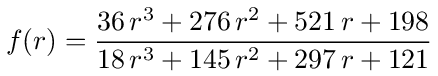
The two extremes are at r=0 and r=∞. We get f(0)=18/11 which is 3 times the parallel combination of a, b and c, or 3/(1 + 1/2 + 1/3)=18/11. We get f(∞)=2 which is 1/3 the series combination of a, b and c, or (1 + 2 + 3)/3=2. The equivalent resistance therefor ranges between 18/11 and 2 as r goes from being a short circuit to an open circuit.
This is a very basic example of software that can be used to implement some of the methods in this book. The software could be greatly improved by using a sparse matrix representation for A. Other improvements would be calculating the frequency response and writing the software in a general purpose programming language like C. The software used in the above examples can be downloaded from the book's website https://www.abrazol.com/books/rwnet/
References & Further Reading
-
Network Analysis, M.E. Van Valkenburg, 3rd ed, 1974.
https://search.worldcat.org/title/693952 -
Passive and Active Network Analysis and Synthesis, Aram Budak, 1974.
https://search.worldcat.org/title/947529 -
Random Walks and Electric Networks, Peter G. Doyle, J. Laurie Snell, 1984.
https://search.worldcat.org/title/11764766 -
Finite Automata and Regular Expressions: Problems and Solutions, Hollos and Hollos, 2013.
https://www.abrazol.com/books/automata/ -
Combinatorics II Problems and Solutions: Counting Patterns, Hollos and Hollos, 2016.
https://www.abrazol.com/books/combinatorics2/
Acknowledgments
In ordinary life we hardly realize that we receive a great deal more
than we give, and that it is only with gratitude that life becomes
rich. It is very easy to overestimate the importance of our own
achievements in comparison with what we owe to others.
Dietrich Bonhoeffer, letter to parents from prison, Sept. 13, 1943
We'd like to thank our parents, Istvan and Anna Hollos, for helping us in many ways.
We thank the makers and maintainers of all the software we've used in the production of this book, including: the Emacs text editor, the LaTex typesetting system, Inkscape, Evince document viewer, Maxima computer algebra system, gcc, bash shell, and the Linux operating system.
About the Authors
Stefan Hollos and J. Richard Hollos are brothers and business partners at Exstrom Laboratories LLC (www.exstrom.com) in Longmont, Colorado. They are physicists and electrical engineers by training, and enjoy anything related to math, physics, engineering and computing. In addition, they enjoy creating music and visual art, and being in the great outdoors. They are the authors of the following books:
- Combinatorics Problems and Solutions, Second Edition
- Creating Noise, second edition
- Engineer's Notebook on Inductor and Transformer Circuits: Problems, Solutions and Simulations
- The Enigma of the Crookes Radiometer
- Passive Butterworth Filter Cookbook
- Nell: An SVG Drawing Language
- Coin Tossing: The Hydrogen Atom of Probability
- Creating Melodies
- Hexagonal Tilings and Patterns
- Combinatorics II Problems and Solutions: Counting Patterns
- Information Theory: A Concise Introduction
- Recursive Digital Filters: A Concise Guide
- Art of Pi
- Creating Noise
- Art of the Golden Ratio
- Creating Rhythms
- Pattern Generation for Computational Art
- Finite Automata and Regular Expressions: Problems and Solutions
- Probability Problems and Solutions
- Combinatorics Problems and Solutions
- The Coin Toss: Probabilities and Patterns
- Pairs Trading: A Bayesian Example
- Simple Trading Strategies That Work
- Bet Smart: The Kelly System for Gambling and Investing
- Signals from the Subatomic World: How to Build a Proton Precession Magnetometer
www.abrazol.com
where you can also sign up for the Abrazol newsletter.
Thank You
Thank you for buying this book.
Sign up for the Abrazol Publishing Newsletter and receive news on
updates, new books, and special offers. Just go to
https://www.abrazol.com/
and enter your email address.
The web page for this book is also located at
abrazol.com