Recursive Digital Filters: A Concise Guide

Simple Low Pass

The first example is a first order low pass filter. First order means that the filter has a single pole which is on the real axis at . The filter also has one zero at . The system function is

$H(z)=\frac{A(z+1)}{z-r}=\frac{A(1+z^{-1})}{1-rz^{-1}}$

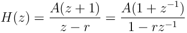(19)

where is a normalization factor chosen so that . A simple calculation shows that . The pole-zero plot is shown in figure 2

Figure 2: Low pass pole-zero plot.

The value of will be large in the vicinity of the pole at and it will be small in the vicinity of the zero at . The frequency response is the magnitude of along the unit circle. The point on the unit circle closest to the pole is which corresponds to zero frequency or DC. This is where the frequency response will be a maximum, which is what you would expect from a low pass filter. The frequency response will have a minimum of zero where which corresponds to the maximum frequency of half the sampling rate.

This is a simple example of how you can use the location of the poles and zeros, with respect to the unit circle, to get a qualitative idea of what the frequency response looks like. Now we’ll look at what a plot of the frequency response magnitude actually looks like. You get a formula for the magnitude by substituting $z=e^{j\theta}$ into eq. 19 and taking the magnitude. After a little algebra and some simplification, the formula is:

$|H(e^{j\theta})|=\frac{(1-r)\cos\frac{\theta}{2}}{\sqrt{1-2r\cos\theta+r^{2}}}$

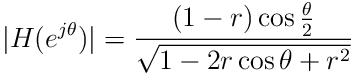(20)

A plot of this for various values of is shown in figure 3.

Figure 3: Low pass frequency response magnitude.

When is close to , the pole is close to the unit circle and the response falls off rapidly as you move away from , i.e. as $\theta$ increases. For smaller values of , the response falls off less rapidly.

To completely characterize this filter we also need to look at the phase of the frequency response. When you substitute $z=e^{j\theta}$ into eq. 19 you can write the frequency response as

$H(e^{j\theta})=|H(e^{j\theta})|e^{j\Phi}$

(21)

We just looked at the equation for the magnitude $|H(e^{j\theta})|$ . Now we want an equation for the phase $\Phi$ . Using the standard procedure for converting a complex expression into polar form, gives the following formula:

$\Phi=\arctan\frac{\sin\theta}{\cos\theta+1}-\arctan\frac{\sin\theta}{\cos% \theta-r}$

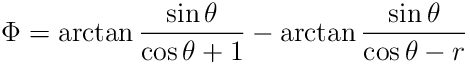(22)

A plot of the phase for various values of is shown in figure 4.

Figure 4: Low pass frequency response phase.

For values of $\theta$ in the pass band of the filter (near ) the phase is almost a linear function of the frequency. This is good because a response with nonlinear phase can cause phase distortion in the signal you are filtering. It’s something to keep in mind but it is often not a problem so we are not going to spend a lot of time on the subject in this introductory treatment of filters.

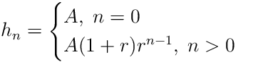
Now let’s look at the impulse response of the filter. To get the impulse response you simply expand as a Taylor series in the variable $z^{-1}$ . You can do this with symbolic math software such as Mathematica or Maxima. This gives

	$\displaystyle H(z)=$	$\displaystyle\frac{A(1+z^{-1})}{1-rz^{-1}}$		(23)
	$\displaystyle=$	$\displaystyle A+A(1+r)(z^{-1}+rz^{-2}+r^{2}z^{-3}+\cdots)$

where is the normalization constant. The $n^{th}$ term in the impulse response is equal to the coefficient of $z^{-n}$ so we have

$h_{n}=\begin{cases}A,\;n=0\\ A(1+r)r^{n-1},\;n>0\end{cases}$

(24)

You can see from this equation that the impulse response only decays if . Only when the pole is inside the unit circle will the filter be stable. It is generally true that the poles of a filter must be inside the unit circle for the filter to be stable.

The filter is implemented by deriving the recursive filter equation from the system function in equation 19. Using in equation 19 and rearranging the terms gives

$(1-rz^{-1})Y(z)=A(1+z^{-1})X(z)$

(25)

which is easily recognized to be the z-transform of the equation

$y_{n}-ry_{n-1}=A(x_{n}+x_{n-1})$

(26)

So the recursive equation for implementing the filter is

$y_{n}=ry_{n-1}+A(x_{n}+x_{n-1})$

(27)

with zero initial conditions, $y_{n}=0$ and $x_{n}=0$ for .

The last question about this filter that we still have to answer is how to choose the value of . will have a large value in the vicinity of the pole at which you can see from the pole-zero plot. When is close to the unit circle, the magnitude of will drop off very rapidly as you move away from along the unit circle. If for some value of $\theta$ we want the magnitude to be reduced to $\alpha<1$ then substitute $|H(e^{j\theta})|=\alpha$ into equation 20 and solve for . This gives

$r=\frac{\alpha^{2}\cos\theta-\cos^{2}\frac{\theta}{2}+\alpha\sqrt{1-\alpha^{2}% }\sin\theta}{\alpha^{2}-\cos^{2}\frac{\theta}{2}}$

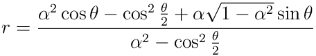(28)

Often times you will have a value of $\theta$ , called the half power point, where you want $\alpha^{2}=1/2$ . In this case equation 28 reduces to

$r=\frac{1-\sin\theta}{\cos\theta}$

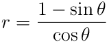(29)

We will show how to use this formula in the following design problem.

Design Problem:

You have a signal that is sampled at samples/sec and you want Hz to be the half power point, i.e. you want all frequencies above Hz to be attenuated by at least a factor of $1/\sqrt{2}=.70710678$ . What value of should you use to accomplish this?

Answer.

The sampling frequency is Hz and the half power frequency is Hz so the dimensionless frequency is $\theta=2\pi f/s=2\pi/10=\pi/5$ . Using this in equation 29 for gives:

$r=\frac{1-\sin\frac{\pi}{5}}{\cos\frac{\pi}{5}}=.509525$

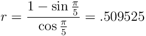
Return to Table of Contents