Introduction
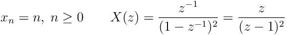
A digital filter takes a series of numbers ![]() as input
and produces the series of numbers
as input
and produces the series of numbers ![]() as output. The
type of filter we are going to talk about is called a linear time
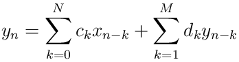
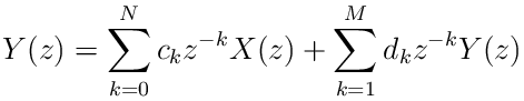
invariant filter. In its most general form the output is related to
the input as follows.
as output. The
type of filter we are going to talk about is called a linear time
invariant filter. In its most general form the output is related to
the input as follows.
|
|
|
(1) | ||
|
|
The equation shows that the current output ![]() is a weighted sum of
the current input
is a weighted sum of
the current input ![]() , the
, the ![]() previous inputs and the
previous inputs and the ![]() previous
outputs. The weight of the
previous
outputs. The weight of the ![]() previous input,
previous input, ![]() , is the
constant
, is the
constant ![]() , and the weight of the
, and the weight of the ![]() previous output,
previous output,
![]() , is the constant
, is the constant ![]() . Equation 1 can be
written more succinctly as
. Equation 1 can be
written more succinctly as
 |
(2) |
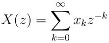
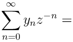
To find out how the filter behaves you have to take the z-transform of
this equation. To take the z-transform of any sequence of numbers
![]() you multiply each
you multiply each ![]() by
by ![]() and sum up all
the products. Assume for now that
and sum up all
the products. Assume for now that ![]() is just some complex number and
let
is just some complex number and
let ![]() be the z-transform of the sequence, then the equation is
be the z-transform of the sequence, then the equation is
 |
(3) |
This definition of the z-transform is usually called the one-sided
z-transform since the summation goes from ![]() to
to ![]() . The full
z-transform takes the summation from
. The full
z-transform takes the summation from ![]() to
to ![]() but we will
only deal with sequences for which
but we will
only deal with sequences for which ![]() for
for ![]() so it becomes
equivalent to the one sided transform in this case.
so it becomes
equivalent to the one sided transform in this case.
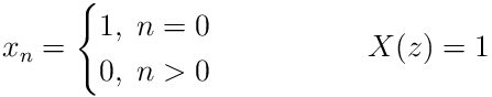
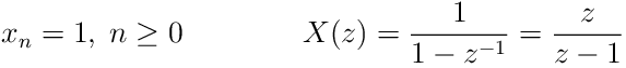
The z-transform is a way to compactly represent a possibly infinite
sequence of numbers. The following are some examples of z-transforms
(in all cases ![]() for
for ![]() ).
).
 |
(4) |
 |
(5) |
 |
(6) |
In general ![]() may not have a simple form as in these examples. If
you are familiar with generating functions then the z-transform looks
like a generating function for the
may not have a simple form as in these examples. If
you are familiar with generating functions then the z-transform looks
like a generating function for the ![]() sequence in the variable
sequence in the variable
![]() and this is essentially what it is. If you are not familiar
with generating functions, don’t worry, they won’t come up again.
and this is essentially what it is. If you are not familiar
with generating functions, don’t worry, they won’t come up again.
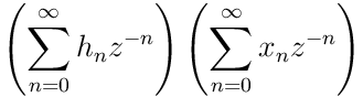
The system function for a digital filter is a z-transform that can be
used to analyze how the filter behaves with different inputs. The
system function will always have the form of the ratio of two
polynomials. To find the system function, multiply both sides of
equation 2 by ![]() and sum over
and sum over ![]() from
from ![]() to
to
![]() . On the left side of the equation, you have
. On the left side of the equation, you have
 |
(7) |
which is the z-transform of the output sequence. On the right side you have terms of the form
 |
For the purpose of describing the operation of a digital filter we can
assume zero initial conditions which simply means that both the ![]() and
and ![]() sequence is zero for
sequence is zero for ![]() . In this case the above equations
are equivalent to
. In this case the above equations
are equivalent to
 |
The summations are the z-transforms of ![]() and
and ![]() so the two
equations are just
so the two
equations are just
Using these results, the z-transform of equation 2 becomes
 |
(8) |
Rearranging the terms in this equation gives you the filter’s system function
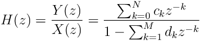 |
(9) |
The system function is the ratio of the z-transform of the output to
the input. By definition ![]() must also be the z-transform of some
sequence which we will call
must also be the z-transform of some
sequence which we will call ![]() . In terms of
. In terms of ![]() , we can write
, we can write
![]() as
as
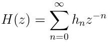 |
(10) |
The sequence ![]() is called the impulse response of the
filter. The name comes from the fact that it is the response of the
filter to the input given by eq. 4 which is called an
impulse. Equation 9 says that
is called the impulse response of the
filter. The name comes from the fact that it is the response of the
filter to the input given by eq. 4 which is called an
impulse. Equation 9 says that ![]() but for
an impulse
but for
an impulse ![]() so we have
so we have ![]() or
or
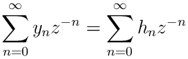 |
(11) |
Equating coefficients of ![]() gives
gives ![]() as the output when
the input is an impulse. For a general sequence of inputs
as the output when
the input is an impulse. For a general sequence of inputs ![]() the output can be found by convolving the inputs with the
impulse response. To see what this means, write
the output can be found by convolving the inputs with the
impulse response. To see what this means, write ![]() as
follows
as
follows
|
|
(12) | ||
|
|
|
|||
|
|
When you perform the multiplication on the right and equate coefficients
of ![]() on the two sides of the equation, you find that
on the two sides of the equation, you find that
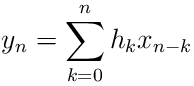 |
(13) |
The summation on the right is called the convolution of the ![]() and
and
![]() sequence. This equation shows why the system function and the
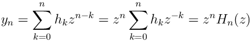
impulse response are so important. Suppose the input is
sequence. This equation shows why the system function and the
impulse response are so important. Suppose the input is ![]() so
that the
so
that the ![]() input is the
input is the ![]() power of the complex number
power of the complex number
![]() . According to eq. 13, the output is then
. According to eq. 13, the output is then
 |
(14) |
The output is the same as the input multiplied by the function
![]() which looks like the system function
which looks like the system function ![]() . It is not
quite the same since the summation only goes to
. It is not
quite the same since the summation only goes to ![]() whereas the system
function summation goes to infinity, as defined in equation
10.
whereas the system
function summation goes to infinity, as defined in equation
10.
But we are only interested in stable filters for which ![]() and
the terms in the impulse response,
and
the terms in the impulse response, ![]() , decrease with increasing
, decrease with increasing ![]() so that
so that ![]() becomes closer and closer to
becomes closer and closer to ![]() as
as ![]() increases, and in the limit
increases, and in the limit ![]() . This means that
after the filter has been running for awhile, its output for the input
. This means that
after the filter has been running for awhile, its output for the input
![]() will, to a good approximation, be
will, to a good approximation, be ![]() .
The filter simply multiplies the input by the factor
.
The filter simply multiplies the input by the factor ![]() to get the
output.
to get the
output.
For inputs of the form ![]() the system function tells you all
you need to know about what the output will be. One important class
of inputs of this form occurs when
the system function tells you all
you need to know about what the output will be. One important class
of inputs of this form occurs when ![]() and
and
![]() . The
. The ![]() are
points on the unit circle in the complex plane (we are using
are
points on the unit circle in the complex plane (we are using
![]() which is the more common convention in engineering
work). An example of such a sequence is shown in figure
1.
which is the more common convention in engineering
work). An example of such a sequence is shown in figure
1.

As the index ![]() increases, the points
increases, the points ![]() move around the unit
circle in angular steps of size
move around the unit
circle in angular steps of size ![]() . The angle
. The angle ![]() acts as
a dimensionless frequency. To see how this can be related to a real
frequency, recall that a periodic function of time,
acts as
a dimensionless frequency. To see how this can be related to a real
frequency, recall that a periodic function of time, ![]() , can
be expressed as a Fourier series which is a weighted sum of the
complex exponentials
, can
be expressed as a Fourier series which is a weighted sum of the
complex exponentials ![]() . When the function is sampled
at intervals
. When the function is sampled
at intervals ![]() then the complex exponentials become
then the complex exponentials become ![]() where
where ![]() ,
, ![]() ,
, ![]() , and
, and ![]() is the sampling rate.
is the sampling rate.
The value of ![]() as
as ![]() ranges from
ranges from ![]() to
to ![]() or
or
![]() to
to ![]() is the frequency response of the filter. In polar
form it can be written as follows
is the frequency response of the filter. In polar
form it can be written as follows
| (15) |
The magnitude ![]() measures how much the filter
amplifies or attenuates the input
measures how much the filter
amplifies or attenuates the input ![]() and the phase
and the phase
![]() measures how much the filter shifts its phase.
measures how much the filter shifts its phase.
Since the value of ![]() will generally be complex, we need
to represent
will generally be complex, we need
to represent ![]() in the complex plane. The simplest way to do that
is with a pole-zero plot.
in the complex plane. The simplest way to do that
is with a pole-zero plot. ![]() will be a rational
function of two polynomials as shown in eq. 9. The
poles of
will be a rational
function of two polynomials as shown in eq. 9. The
poles of ![]() are those values of
are those values of ![]() where
where ![]() goes to infinity.
These values are the roots of the denominator polynomial, and
goes to infinity.
These values are the roots of the denominator polynomial, and
![]() if the numerator degree is greater than the denominator
degree. The zeros of
if the numerator degree is greater than the denominator
degree. The zeros of ![]() are those values of
are those values of ![]() where
where ![]() is
zero. These values are the roots of the numerator polynomial, and
is
zero. These values are the roots of the numerator polynomial, and
![]() if the denominator degree is greater than the numerator
degree. A pole-zero plot of
if the denominator degree is greater than the numerator
degree. A pole-zero plot of ![]() simply shows the location of the
poles and zeros in the complex plane along with the unit circle.
Poles are represented by a filled circle “
simply shows the location of the
poles and zeros in the complex plane along with the unit circle.
Poles are represented by a filled circle “![]() ”, and zeros by an
unfilled circle “
”, and zeros by an
unfilled circle “![]() ”.
”.
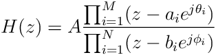
Let the the zeros of ![]() be
be ![]() ,
, ![]() , and the poles
be
, and the poles
be ![]() ,
, ![]() , then
, then ![]() can be written as
can be written as
 |
(16) |
In eq. 9 the coefficients of the numerator and
denominator polynomial are real. For the filters we will consider,
this will always be true. This means that complex poles or zeros must
come in conjugate pairs. If ![]() is a complex zero then
there must be another zero equal to
is a complex zero then
there must be another zero equal to ![]() and likewise for
poles.
and likewise for
poles.
Substituting ![]() into equation 16 and
taking the magnitude and phase gives the following equations
into equation 16 and
taking the magnitude and phase gives the following equations
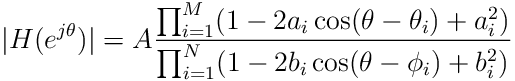 |
(17) |
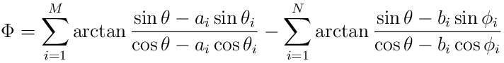 |
(18) |
The following sections will show how these equations are used.
Return to Table of Contents